Brief Summary
This lecture by Professor Leonard introduces the fundamental concepts of calculus, focusing on limits, tangents, and areas under curves. It explains the two primary goals of calculus: finding the slope of a curve at a point (the tangent problem) and determining the area under a curve between two points (the area problem). The lecture uses the concept of limits to transition from secant lines to tangent lines and introduces one-sided limits to determine when a limit exists.
- Introduction to Calculus and Limits
- Tangent and Area Problems
- One-Sided Limits and Existence of Limits
Introduction to Calculus and Limits
The lecture begins by emphasizing the importance of limits as the foundation of calculus. It outlines two main goals: finding the slope of a curve at a specific point and calculating the area under a curve between two points. These problems are impossible to solve using algebra alone, making calculus necessary. The first goal, finding the tangent to a curve, involves determining the slope at a single point, which leads to the concept of a tangent line intersecting the curve at only one spot in a local area. The second goal involves finding the area under a curve, which cannot be done with standard geometric formulas due to the curve's irregular shape.
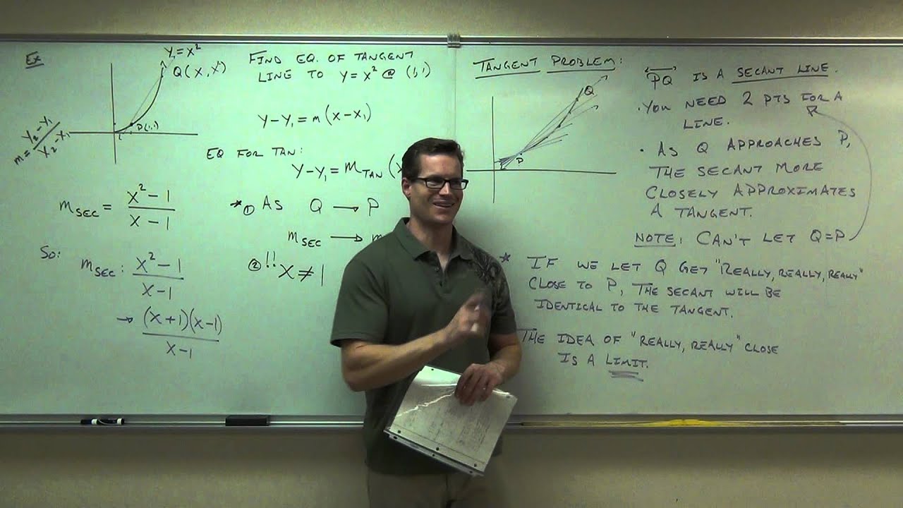
The Tangent Problem: Secants and Approximations
The lecture introduces the tangent problem, which aims to find the slope of a curve at a given point P. Since defining a line requires two points, a secant line is drawn through point P and another point Q on the curve. The goal is to approximate the tangent line by moving point Q closer to point P. As Q approaches P, the secant line becomes a better approximation of the tangent line. However, Q cannot equal P because two distinct points are needed to define a line. The idea of a limit is introduced as the concept of getting Q infinitely close to P without them being the same point, making the secant line virtually identical to the tangent line.
Limits: Getting Infinitely Close
The core idea of a limit is explored: how close can one point get to another without coinciding? This concept is crucial for calculus because it allows mathematicians to consider values that are nearly equal without actually being equal. The lecture explains that by letting Q get infinitely close to P, the secant line becomes indistinguishable from the tangent line. This "really, really close" concept is formalized as a limit, where Q approaches P without ever touching it.
Example: Finding the Tangent Line
Professor Leonard provides a detailed example to find the equation of the tangent line to the curve y = x² at the point (1,1). A movable point Q (x, x²) is introduced to create a secant line with point P (1,1). The slope of the secant line is calculated using the slope formula: (x² - 1) / (x - 1). The lecture then addresses the issue that plugging in x = 1 results in an undefined expression (0/0). To resolve this, the expression is factored and simplified to x + 1, with the understanding that x is approaching 1 but not equal to 1. By making x get closer to 1, the slope of the secant line approaches 2, which is then taken as the slope of the tangent line. The equation of the tangent line is found to be y = 2x - 1.
The Area Problem: Approximating with Rectangles
The lecture transitions to the area problem, which involves finding the area under a curve between two points. Since curves cannot be directly measured for area, the solution involves approximating the area using rectangles. By creating multiple rectangles under the curve, the area can be estimated. The more rectangles used, the better the approximation. The ideal solution involves using an infinite number of infinitesimally small rectangles to achieve a perfect area calculation. This process also involves limits, as the number of rectangles approaches infinity.
Defining Limits: Approaching a Value
A limit is defined as what a function does as a variable approaches a given value, not what the function's value is at that specific point. An example is provided using the function f(x) = x² as x approaches 2. A table is created with values approaching 2 from both the left and the right to observe the function's behavior. The function must approach the same value from both sides for the limit to exist. In this case, as x approaches 2, f(x) approaches 4.
One-Sided Limits: Left and Right Approaches
The concept of one-sided limits is introduced, distinguishing between approaching a value from the right (denoted with a superscript plus sign) and from the left (denoted with a superscript minus sign). For a limit to exist at a point, the left-sided limit must equal the right-sided limit. Several examples using graphs are provided to illustrate how to determine one-sided limits and whether a limit exists based on these one-sided limits.
Limits and Asymptotes: Approaching Infinity
The lecture explores limits that approach infinity, particularly in the context of the function 1/x as x approaches 0. It's shown that as x approaches 0 from the right, the function goes to positive infinity, and as x approaches 0 from the left, the function goes to negative infinity. This leads to the concept of asymptotes. If a limit as x approaches a (from either the right or left) results in positive or negative infinity, there is an asymptote at x = a. The lecture concludes by illustrating the four possible cases of asymptotes and their corresponding limits.